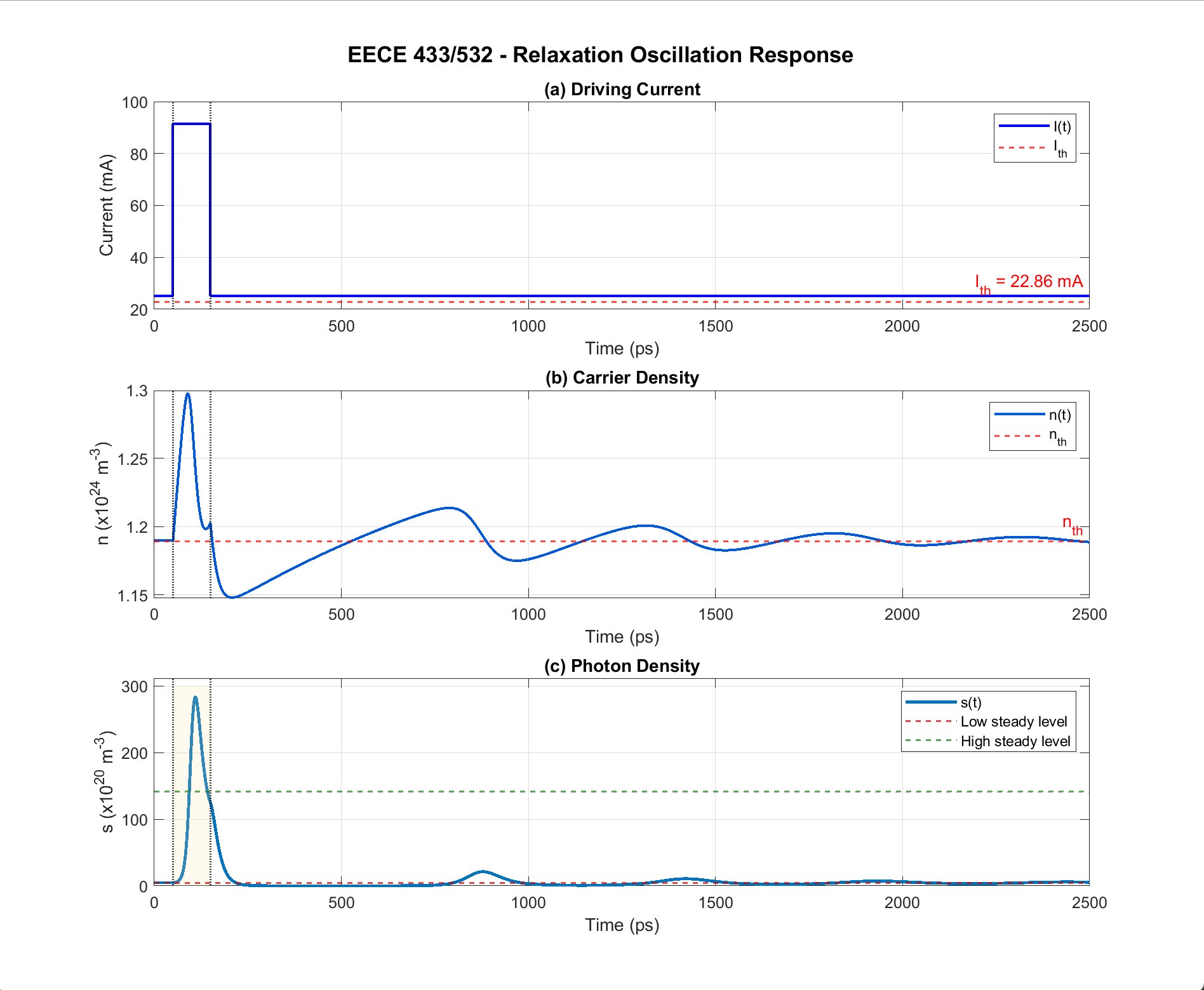
Semiconductor Laser Relaxation Oscillations

Numerical simulation of a directly modulated semiconductor laser using coupled rate equations for carrier and photon density. The device is biased just above threshold, pulsed to a higher drive current for 100 ps, then returned to bias. This is the same scenario a laser sees under direct modulation in a data link.

Rate equations

Carrier and photon densities are coupled through a gain term that includes compression:

\[ \frac{dn}{dt} = \frac{I}{qV} - \frac{n}{\tau} - \Gamma\, G(n,s)\, s \] \[ \frac{ds}{dt} = \Gamma\, G(n,s)\, s - \frac{s}{\tau_p} + \beta\, \frac{n}{\tau} \] \[ G(n,s) = \frac{v_g \,(dg/dn)\,(n - n_0)}{1 + \varepsilon s} \]

Device parameters

Parameter	Symbol	Value
Active region volume	\(V\)	\(120\ \mu\mathrm{m}^3\)
Photon lifetime	\(\tau_p\)	\(4\ \mathrm{ps}\)
Carrier lifetime	\(\tau\)	\(1\ \mathrm{ns}\)
Spontaneous emission factor	\(\beta\)	\(10^{-5}\)
Differential gain	\(dg/dn\)	\(5\times10^{-16}\ \mathrm{cm}^2\)
Gain compression	\(\varepsilon\)	\(10^{-17}\ \mathrm{cm}^3\)
Confinement factor	\(\Gamma\)	\(0.30\)
Transparency carrier density	\(n_0\)	\(10^{18}\ \mathrm{cm}^{-3}\)

Results

Threshold came out to \(n_{\mathrm{th}} \approx 1.19 \times 10^{18}\ \mathrm{cm}^{-3}\) and \(I_{\mathrm{th}} \approx 22.9\ \mathrm{mA}\). Steady state at \(1.1\,I_{\mathrm{th}}\) was found by integrating to convergence over 8 ns rather than assuming carrier clamping, so the transient starts from a self-consistent bias point.

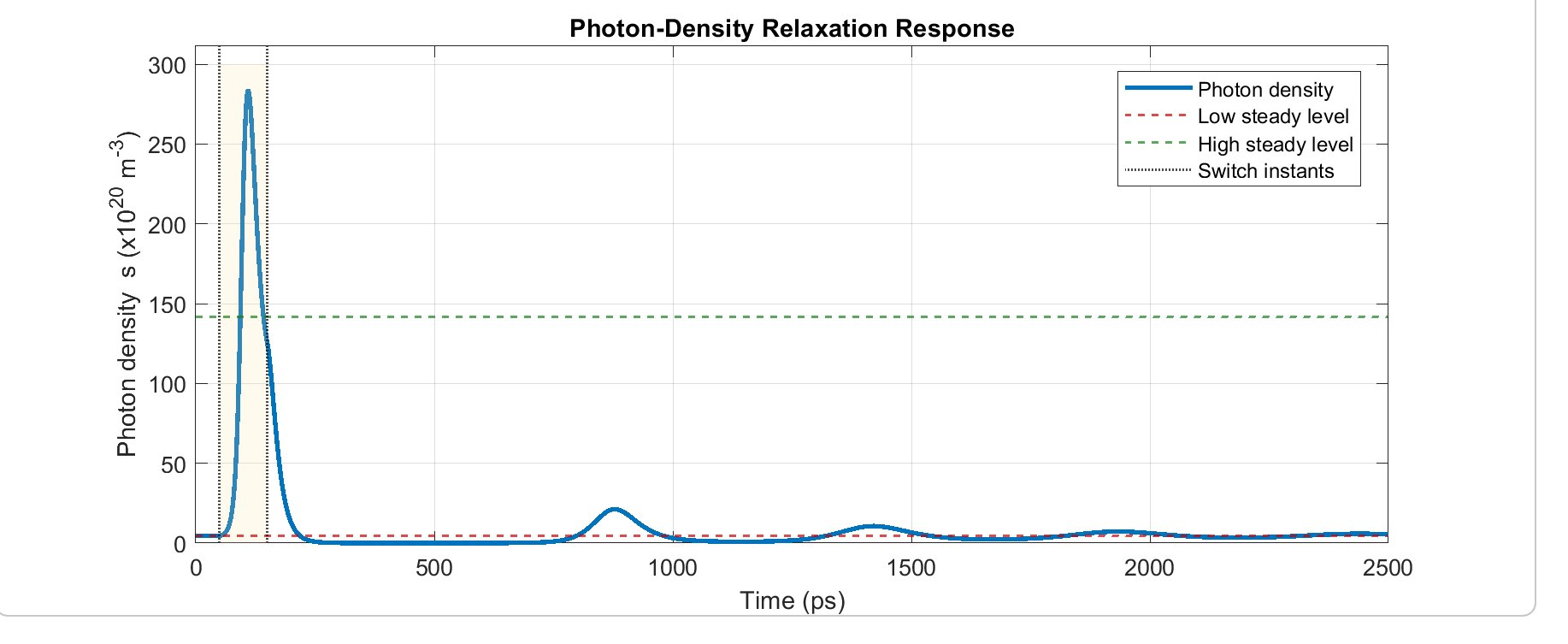
When the current steps up, carrier density overshoots \(n_{\mathrm{th}}\) before stimulated emission can respond. Once photon density spikes it clamps the carriers, triggering a damped oscillatory exchange, plus a second burst on the step back down. Relaxation oscillation frequency for this parameter set landed at ~5 to 15 GHz.

Three stacked plots showing driving current, carrier density, and photon density versus time over 2500 picoseconds — Driving current, carrier density, and photon density vs. time. The 100 ps pulse window is shaded; damped relaxation oscillations are visible in both n(t) and s(t) after each edge.

Photon density versus time plot in eye-pattern style, showing the pulse spike and steady-state levels — Photon-density response in eye-pattern style, with low and high steady-state levels marked.

MATLAB source: rate equations and threshold

% Part (a): Threshold current
% Threshold condition: Gamma * vg * dgdn * (nth - n0) = 1/tau_p
delta_nth = 1 / (Gamma * vg * dgdn * tau_p);
nth  = n0 + delta_nth;
I_th = q * V * nth / tau;

% Transient: 1.1*Ith -> 4*Ith for 100 ps -> back to 1.1*Ith
I_func = @(t) I_bias + (I_high - I_bias) * (t >= t_on & t <= t_off);

opts   = odeset('RelTol', 1e-8, 'AbsTol', 1e-10, 'MaxStep', 0.2e-12);
t_eval = linspace(0, t_end, 8000);
[t_sol, y_sol] = ode45(@(t, y) rate_eqs(t, y, I_func, q, V, tau, tau_p, ...
    beta, Gamma, vg, dgdn, n0, epsilon), t_eval, y0, opts);

function dydt = rate_eqs(t, y, I_func, q, V, tau, tau_p, beta, ...
                         Gamma, vg, dgdn, n0, epsilon)
    n = max(y(1), 0);
    s = max(y(2), 0);
    I = I_func(t);
    G = vg * dgdn * (n - n0) / (1 + epsilon * s);
    dndt = I/(q*V) - n/tau - Gamma*G*s;
    dsdt = Gamma*G*s - s/tau_p + beta*n/tau;
    dydt = [dndt; dsdt];
end

MATLABode45 Rate equationsGain compression Direct modulationLaser dynamics

View on GitHub